Sort phyloseq samples by ordination axes scores

ps_sort_ord reorders samples in a phyloseq object based on their relative position on 1 or 2 ordination axes.

ord_order_samples gets the sample_names in order from the ordination contained in a psExtra. This is used internally by ps_sort_ord

If 2 axes given, the samples are sorted by anticlockwise rotation around the selected ordination axes, starting on first axis given, upper right quadrant. (This is used by ord_plot_iris.)

If 1 axis is given, samples are sorted by increasing value order along this axis. This could be used to arrange samples on a rectangular barplot in order of appearance along a parallel axis of a paired ordination plot.

ps_sort_ord(ps, ord, axes = 1:2, scaling = 2)

ord_order_samples(ord, axes = 1:2, scaling = 2)

Arguments

ps: phyloseq object to be sorted
ord: psExtra with ordination object
axes: which axes to use for sorting? numerical vector of length 1 or 2
scaling: Type 2, or type 1 scaling. For more info, see https://sites.google.com/site/mb3gustame/constrained-analyses/redundancy-analysis. Either "species" or "site" scores are scaled by (proportional) eigenvalues, and the other set of scores is left unscaled (from ?vegan::scores.cca)

Value

ps_sort_ord returns a phyloseq

ord_order_samples returns a character vector

Examples

# attach other necessary packages
library(ggplot2)

# example data
ibd <- microViz::ibd %>%
  tax_filter(min_prevalence = 2) %>%
  tax_fix() %>%
  phyloseq_validate()

# create numeric variables for constrained ordination
ibd <- ibd %>%
  ps_mutate(
    ibd = as.numeric(ibd == "ibd"),
    steroids = as.numeric(steroids == "steroids"),
    abx = as.numeric(abx == "abx"),
    female = as.numeric(gender == "female"),
    # and make a shorter ID variable
    id = stringr::str_remove_all(sample, "^[0]{1,2}|-[A-Z]+")
  )

# create an ordination
ordi <- ibd %>%
  tax_transform("clr", rank = "Genus") %>%
  ord_calc()

ord_order_samples(ordi, axes = 1) %>% head(8)
#> [1] "048A" "051A" "025A" "199A" "200A" "218A" "119A" "210A"
ps_sort_ord(ibd, ordi, axes = 1) %>%
  phyloseq::sample_names() %>%
  head(8)
#> [1] "048A" "051A" "025A" "199A" "200A" "218A" "119A" "210A"

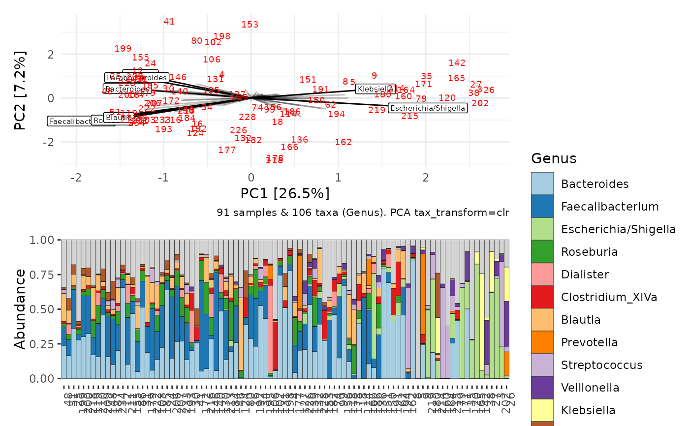
p1 <- ord_plot(ordi, colour = "grey90", plot_taxa = 1:8, tax_vec_length = 1) +
  geom_text(aes(label = id), size = 2.5, colour = "red")

b1 <- ibd %>%
  ps_sort_ord(ord = ordi, axes = 1) %>%
  comp_barplot(
    tax_level = "Genus", n_taxa = 12, label = "id",
    order_taxa = ord_order_taxa(ordi, axes = 1),
    sample_order = "asis"
  ) +
  theme(axis.text.x = element_text(angle = 90, hjust = 1))

patchwork::wrap_plots(p1, b1, ncol = 1)


# constrained ordination example (and match vertical axis) #
cordi <- ibd %>%
  tax_transform("clr", rank = "Genus") %>%
  ord_calc(
    constraints = c("steroids", "abx", "ibd"), conditions = "female",
    scale_cc = FALSE
  )

cordi %>% ord_plot(plot_taxa = 1:6, axes = 2:1)

Sort phyloseq samples by ordination axes scores

Arguments

Value

See also

Examples