Intro
This article will show you how to create and customise ordination plots, like PCA and RDA, with microViz.
For an even quicker start with ordinating your phyloseq data, check
out the ord_explore Shiny
app, which allows you to create ordination plots with a point and
click interface, and generates ord_plot code for you to
copy. Return to this article to understand more about creating and
customising your ordination plotting script.
library(phyloseq)
library(ggplot2)
library(microViz)
#> microViz version 0.13.1 - Copyright (C) 2021-2026 David Barnett
#> ! Website: https://david-barnett.github.io/microViz
#> ✔ Useful?  For citation details, run: `citation("microViz")`
#> ✖ Silence? `suppressPackageStartupMessages(library(microViz))`
knitr::opts_chunk$set(fig.width = 7, fig.height = 6)
We will use example data from stool samples from an inflammatory
bowel disease (IBD) study, borrowed from the great corncob
package. See the article about working
with phyloseq objects if you want to get started with your own data,
or just to learn more about manipulating phyloseq objects with
microViz.
ibd <- microViz::ibd
ibd
#> phyloseq-class experiment-level object
#> otu_table()   OTU Table:         [ 36349 taxa and 91 samples ]
#> sample_data() Sample Data:       [ 91 samples by 15 sample variables ]
#> tax_table()   Taxonomy Table:    [ 36349 taxa by 7 taxonomic ranks ]
First we fix any uninformative tax_table entries and check the phyloseq object (see the article on fixing your tax_table for more info).
ibd <- tax_fix(ibd) # try tax_fix_interactive if you have problems with your own data
ibd <- phyloseq_validate(ibd, remove_undetected = TRUE)
Motivation
Ordination plots are a great way to see any clustering or other
patterns of microbiota (dis)similarity in (many) samples. Ordinations
like PCA or PCoA show the largest patterns of variation in your data,
and constrained ordination techniques like RDA or CCA can show you
microbial variation that could be explained by other variables in your
sample_data (but interpret constrained ordinations with care, and
ideally test for the statistical significance of any hypothesised
associations using a method like PERMANOVA, see
dist_permanova()).
Check out the GUide to STatistical Analysis in Microbial Ecology (GUSTA ME)website for a gentle theoretical introduction to PCA, PCoA, RDA, CCA and more.
Ordination plots can also be paired with barplots for greater insight
into microbial compositions, e.g. see ord_plot_iris() and
the ord_explore() interactive Shiny
app.
Prepare your microbes
When creating an ordination plot, you first need to prepare the microbiota variables.
Decide at which taxonomic rank to aggregate your data, e.g. “Genus”
Consider transforming the microbial counts, e.g. using the “clr” (centred log ratio) transformation, which is often recommended for compositional data (like sequencing data)
ibd %>%
  tax_transform(trans = "clr", rank = "Genus")
#> psExtra object - a phyloseq object with extra slots:
#>
#> phyloseq-class experiment-level object
#> otu_table()   OTU Table:         [ 178 taxa and 91 samples ]
#> sample_data() Sample Data:       [ 91 samples by 15 sample variables ]
#> tax_table()   Taxonomy Table:    [ 178 taxa by 6 taxonomic ranks ]
#>
#> otu_get(counts = TRUE)        [ 178 taxa and 91 samples ]
#>
#> psExtra info:
#> tax_agg = "Genus" tax_trans = "clr"- Some methods, such as PCoA, require a matrix of
pairwise distances between samples, which you can easily calculate with
dist_calc(). Normally you should NOT transform your data when using a distance-based method, but it is useful to record an “identity” transformation anyway, to make it clear you have not transformed your data.
ibd %>%
  tax_transform(trans = "identity", rank = "Genus") %>%
  dist_calc("bray") # bray curtis distance
#> psExtra object - a phyloseq object with extra slots:
#>
#> phyloseq-class experiment-level object
#> otu_table()   OTU Table:         [ 178 taxa and 91 samples ]
#> sample_data() Sample Data:       [ 91 samples by 15 sample variables ]
#> tax_table()   Taxonomy Table:    [ 178 taxa by 6 taxonomic ranks ]
#>
#> psExtra info:
#> tax_agg = "Genus" tax_trans = "identity"
#>
#> bray distance matrix of size 91
#> 0.8294664 0.7156324 0.5111652 0.5492537 0.8991251 ...- Some dissimilarity measures, such as unweighted UniFrac, do not
consider the abundance of each taxon when calculating dissimilarity, and
so may be (overly) sensitive to differences in rare/low-abundance taxa.
So you might want to filter out very rare taxa, with
tax_filter()before usingdist_calc(ps, dist = "unifrac"). Distances that are (implicitly) abundance weighted, including Generalised UniFrac, Bray-Curtis and Aitchison distance, should be less sensitive to rare taxa / filtering threshold choices.
psExtra
Notice that the objects created above are of class “psExtra”. This is
an S4 class object that holds your phyloseq object with additional slots
for stuff created from this phyloseq object, such as a distance matrix,
as well as info on any transformation and aggregation applied to your
taxa. microViz uses this to automatically create plot captions, to help
you and your collaborators remember how you made each plot! You can
access the phyloseq object, distance matrix and other parts of a psExtra
object with ps_get(), dist_get(), and
friends.
PCA - Principal Components Analysis
Principal Components Analysis is an
unconstrained method that does not use a distance matrix. PCA directly
uses the (transformed) microbial variables, so you do not need
dist_calc(). ord_calc performs the ordination
(adding it to the psExtra object) and ord_plot() creates
the ggplot2 scatterplot (which you can customise like other ggplot
objects).
Each point is a sample, and samples that appear closer together are typically more similar to each other than samples which are further apart. So by colouring the points by IBD status you can see that the microbiota from people with IBD is often, but not always, highly distinct from people without IBD.
ibd %>%
  tax_transform("clr", rank = "Genus") %>%
  # when no distance matrix or constraints are supplied, PCA is the default/auto ordination method
  ord_calc() %>%
  ord_plot(color = "ibd", shape = "DiseaseState", size = 2) +
  scale_colour_brewer(palette = "Dark2")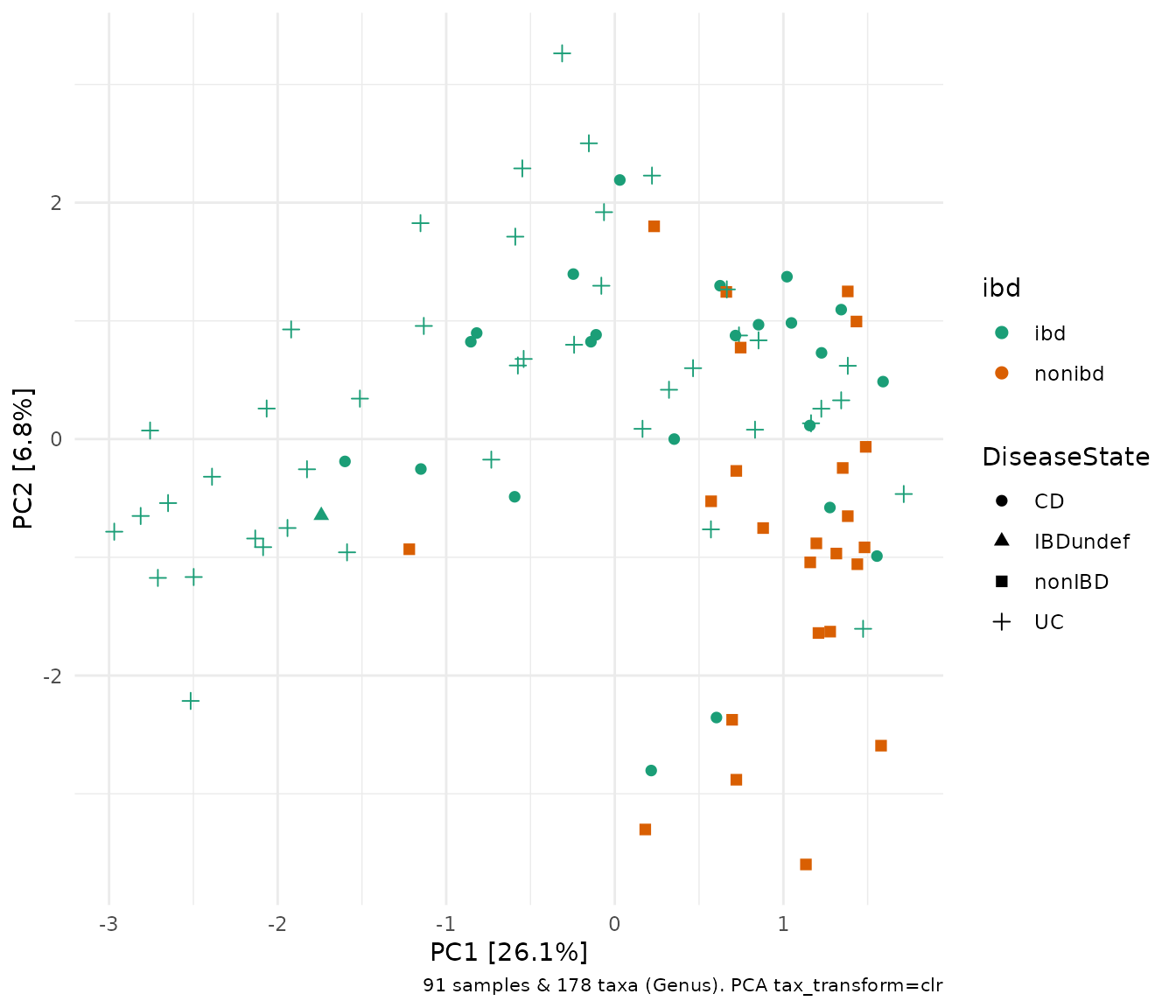
One benefit of not using a distance matrix, is that you can plot taxa “loadings” onto your PCA axes, using the plot_taxa argument. microViz plots all of the taxa loading vectors in light grey, and you choose how many of the vectors to label, starting with the longest arrows (alternatively you can name particular taxa to label).
The relative length of each loading vector indicates its contribution to each PCA axis shown, and allows you to roughly estimate which samples will contain more of that taxon e.g. samples on the left of the plot below, will typically contain more Escherichia/Shigella than samples on the right, and this taxon contributes heavily to the PC1 axis.
ibd %>%
  tax_transform("clr", rank = "Genus") %>%
  # when no distance matrix or constraints are supplied, PCA is the default/auto ordination method
  ord_calc(method = "PCA") %>%
  ord_plot(color = "ibd", shape = "DiseaseState", plot_taxa = 1:5, size = 2) +
  scale_colour_brewer(palette = "Dark2")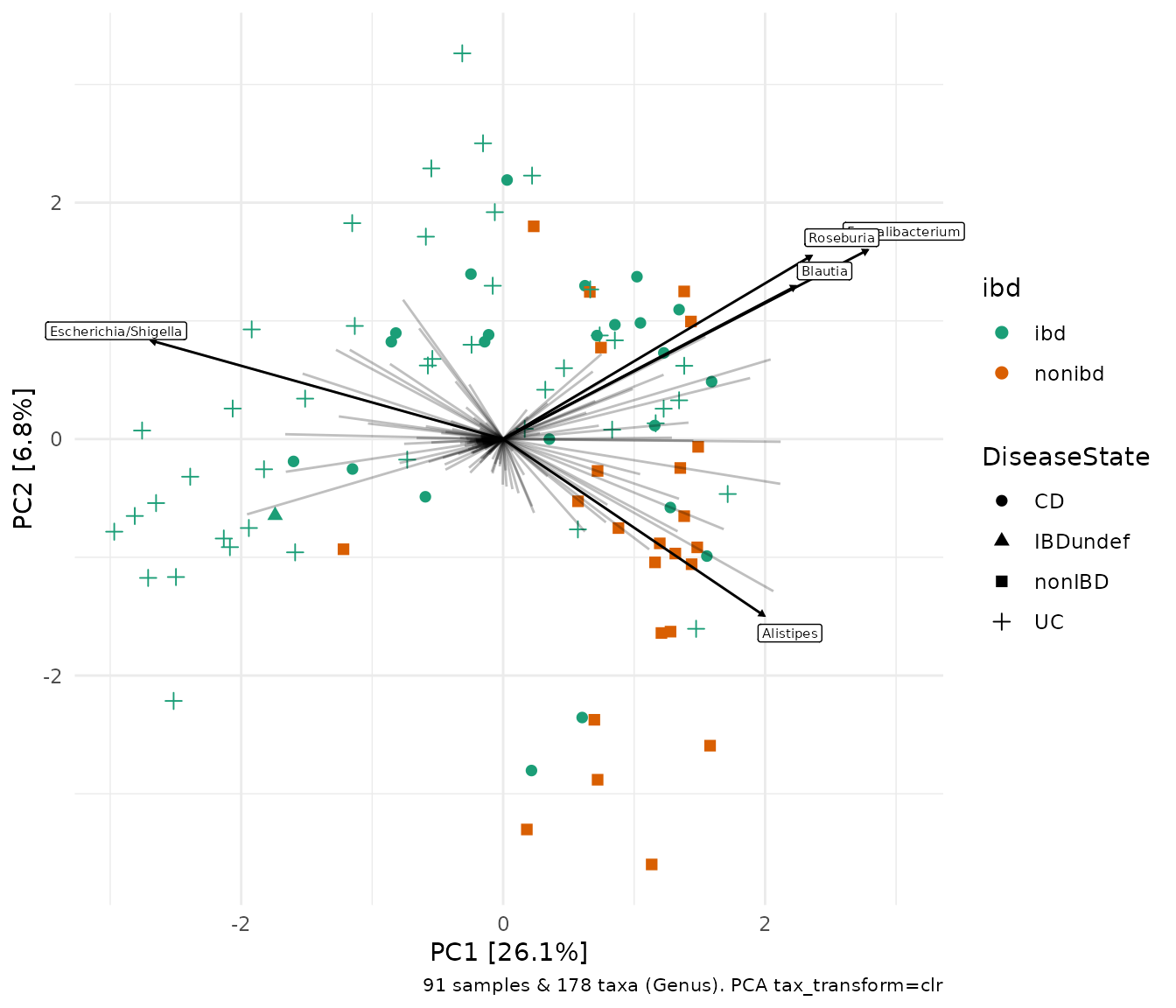
microViz also allows you directly visualize the sample compositions on a circular barplot or “iris plot” (named because it looks kinda like an eyeball) alongside the PCA plot. The samples on the iris plot are automatically arranged by their rotational position around the center/origin of the PCA plot.
ibd %>%
  tax_transform("clr", rank = "Genus") %>%
  # when no distance matrix or constraints are supplied, PCA is the default/auto ordination method
  ord_calc() %>%
  ord_plot_iris(tax_level = "Genus", ord_plot = "above", anno_colour = "ibd")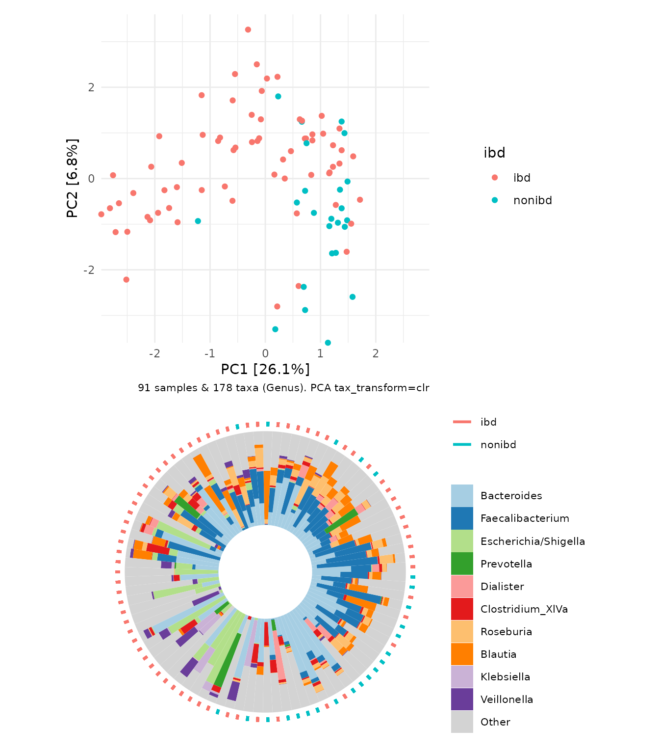
Here we created the ordination plot as a quick accompaniment to the
circular barchart, but it is more flexible to create and customise the
ordination plot and iris plot separately, and then pair them afterwards
with patchwork. See the ord_plot_iris docs
for examples.
PCoA - Principal Co-ordinates Analysis
Principal Co-ordinates Analysis is also an unconstrained method, but it does require a distance matrix. In an ecological context, a distance (or more generally a “dissimilarity”) measure indicates how different a pair of (microbial) ecosystems are. This can be calculated in many ways.
Aitchison distance
The Euclidean distance is similar to the distance we humans are familiar with in the physical world. The results of a PCA is practically equivalent to a PCoA with Euclidean distances. The Aitchison distance is a dissimilarity measure calculated as the Euclidean distance between observations (samples) after performing a centered log ratio (“clr”) transformation. That is why the Aitchison distance PCoA, below, looks the same as the PCA we made earlier. However, we cannot use plot_taxa, as the taxa loadings are only available for PCA (and related methods like RDA).
ibd %>%
  tax_transform("identity", rank = "Genus") %>% # don't transform!
  dist_calc("aitchison") %>%
  ord_calc("PCoA") %>%
  ord_plot(color = "ibd", shape = "DiseaseState", size = 2) +
  scale_colour_brewer(palette = "Dark2")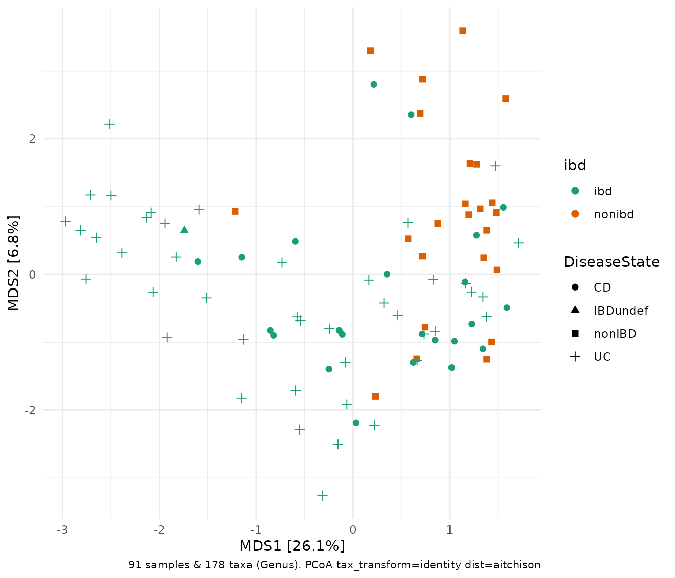
Note that PCoA is also known as MDS, for (metric) Multi-Dimensional Scaling, hence the axes names.
Ecological dissimilarities
Over the years, ecologists have invented numerous ways of quantifying dissimilarity between pairs of ecosystems. One ubiquitous example is the Bray-Curtis dissimilarity measure, shown below.
ibd %>%
  tax_transform("identity", rank = "Genus") %>% # don't transform!
  dist_calc("bray") %>%
  ord_calc("PCoA") %>%
  ord_plot(color = "ibd", shape = "DiseaseState", size = 2) +
  scale_colour_brewer(palette = "Dark2")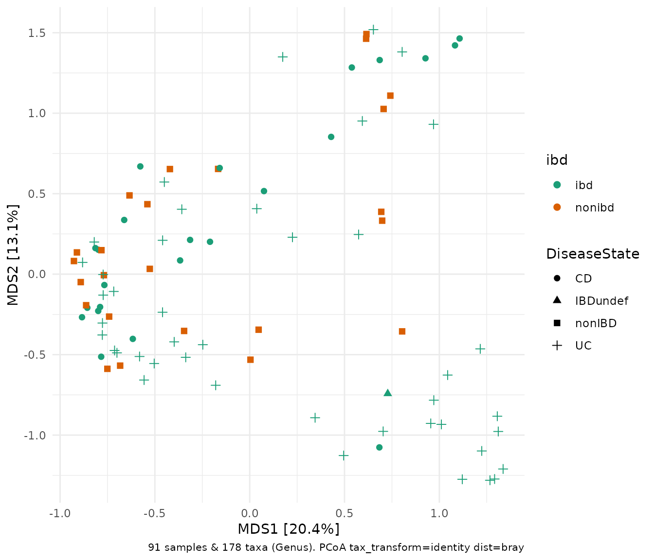
Beyond Bray-Curtis, microViz dist_calc() can also help
you calculate all the other ecological distances listed in
phyloseq::distanceMethodList such the Jensen-Shannon
Divergence, "jsd", or Jaccard dissimilarity
"jaccard". Beware that if you want a binary dissimilarity
measure from vegan::vegdist() (i.e. only using
presence/absence info, and noting all the caveats about sensitivity to
low abundance taxa) you will need to pass binary = TRUE, as
below.
ibd %>%
  tax_transform("identity", rank = "Genus") %>%
  dist_calc(dist = "jaccard", binary = TRUE) %>%
  ord_calc("PCoA") %>%
  ord_plot(color = "ibd", shape = "DiseaseState", size = 2) +
  scale_colour_brewer(palette = "Dark2")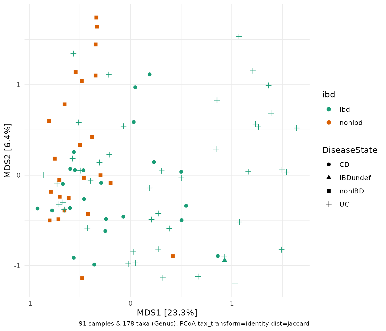
UniFrac distances
If you have a phylogenetic tree available, and attached
to your phyloseq object. You can calculate dissimilarities from the
UniFrac family of
methods, which take into account the phylogenetic relatedness of the
taxa / sequences in your samples when calculating dissimilarity.
Un-weighted UniFrac, dist_calc(dist = "unifrac"), does not
consider the relative abundance of taxa, only their presence (detection)
or absence, which can make it (overly) sensitive to rare taxa,
sequencing artefacts, and abundance filtering choices. Conversely,
weighted UniFrac, "wunifrac", does put (perhaps too much)
more importance on highly abundant taxa, when determining
dissimilarities. The Generalised UniFrac, "gunifrac", finds
a balance between these two extremes, and by adjusting the
gunifrac_alpha argument of dist_calc(), you
can tune this balance to your liking (although the 0.5 default should be
fine!).
Below is a Generalised UniFrac example using a different, and tiny, example dataset from the phyloseq package that has a phylogenetic tree.
You should not aggregate taxa before using a phylogenetic distance measure, but you can and probably should register the choice not to transform or aggregate, as below.
data("esophagus", package = "phyloseq")
esophagus %>%
  phyloseq_validate(verbose = FALSE) %>%
  tax_transform("identity", rank = "unique") %>%
  dist_calc("gunifrac", gunifrac_alpha = 0.5)
#> psExtra object - a phyloseq object with extra slots:
#>
#> phyloseq-class experiment-level object
#> otu_table()   OTU Table:         [ 58 taxa and 3 samples ]
#> sample_data() Sample Data:       [ 3 samples by 1 sample variables ]
#> tax_table()   Taxonomy Table:    [ 58 taxa by 1 taxonomic ranks ]
#> phy_tree()    Phylogenetic Tree: [ 58 tips and 57 internal nodes ]
#>
#> psExtra info:
#> tax_agg = "unique" tax_trans = "identity"
#>
#> gunifrac_0.5 distance matrix of size 3
#> 0.4404284 0.4332325 0.4969773 ...
Further dimensions
You can show other dimensions / axes of an ordination than just the first two, by setting the axes argument. You can judge from the variation explained by each successive axis (on a scree plot) whether this is worthwhile information to show, e.g. in the example below, it could be interesting to also show the 3rd axis, but not any others.
ibd %>%
  tax_transform("identity", rank = "Genus") %>% # don't transform!
  dist_calc("bray") %>%
  ord_calc("PCoA") %>%
  ord_get() %>%
  phyloseq::plot_scree() + theme(axis.text.x = element_text(size = 6))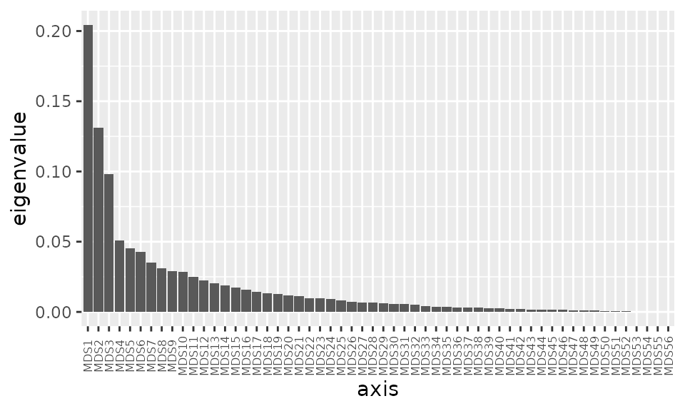
Let us view the 1st and 3rd axes.
ibd %>%
  tax_transform("identity", rank = "Genus") %>% # don't transform!
  dist_calc("bray") %>%
  ord_calc("PCoA") %>%
  ord_plot(axes = c(1, 3), color = "ibd", shape = "DiseaseState", size = 2) +
  scale_colour_brewer(palette = "Dark2")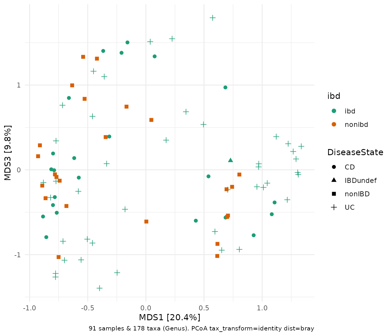
Univariable distribution side panels
As the ordination figures are (pretty much) just standard ggplot
objects, integration with other ggplot extensions like
ggside is typically possible. Below are a couple of
examples using the ggside package to add univariable
distribution plots for each PC, split by the same groups as in the main
plot.
Side panel boxplots
ibd %>%
  tax_transform("identity", rank = "Genus") %>%
  dist_calc(dist = "aitchison") %>%
  ord_calc("PCoA") %>%
  ord_plot(color = "ibd", shape = "DiseaseState", size = 2) +
  scale_colour_brewer(palette = "Dark2", aesthetics = c("fill", "colour")) +
  theme_bw() +
  ggside::geom_xsideboxplot(aes(fill = ibd, y = ibd), orientation = "y") +
  ggside::geom_ysideboxplot(aes(fill = ibd, x = ibd), orientation = "x") +
  ggside::scale_xsidey_discrete(labels = NULL) +
  ggside::scale_ysidex_discrete(labels = NULL) +
  ggside::theme_ggside_void()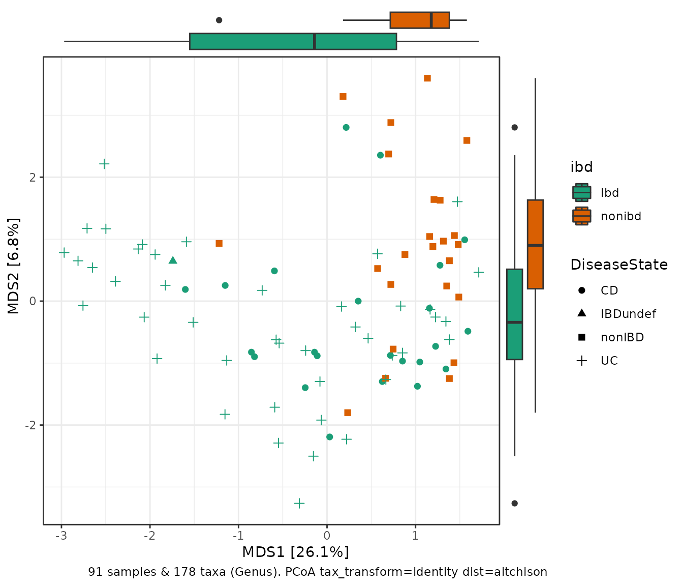
Side panel density plots
ibd %>%
  tax_transform("identity", rank = "Genus") %>%
  dist_calc(dist = "aitchison") %>%
  ord_calc("PCoA") %>%
  ord_plot(color = "ibd", shape = "DiseaseState", size = 2) +
  scale_colour_brewer(palette = "Dark2", aesthetics = c("fill", "colour"), name = "IBD") +
  theme_bw() +
  ggside::geom_xsidedensity(aes(fill = ibd), alpha = 0.5, show.legend = FALSE) +
  ggside::geom_ysidedensity(aes(fill = ibd), alpha = 0.5, show.legend = FALSE) +
  ggside::theme_ggside_void()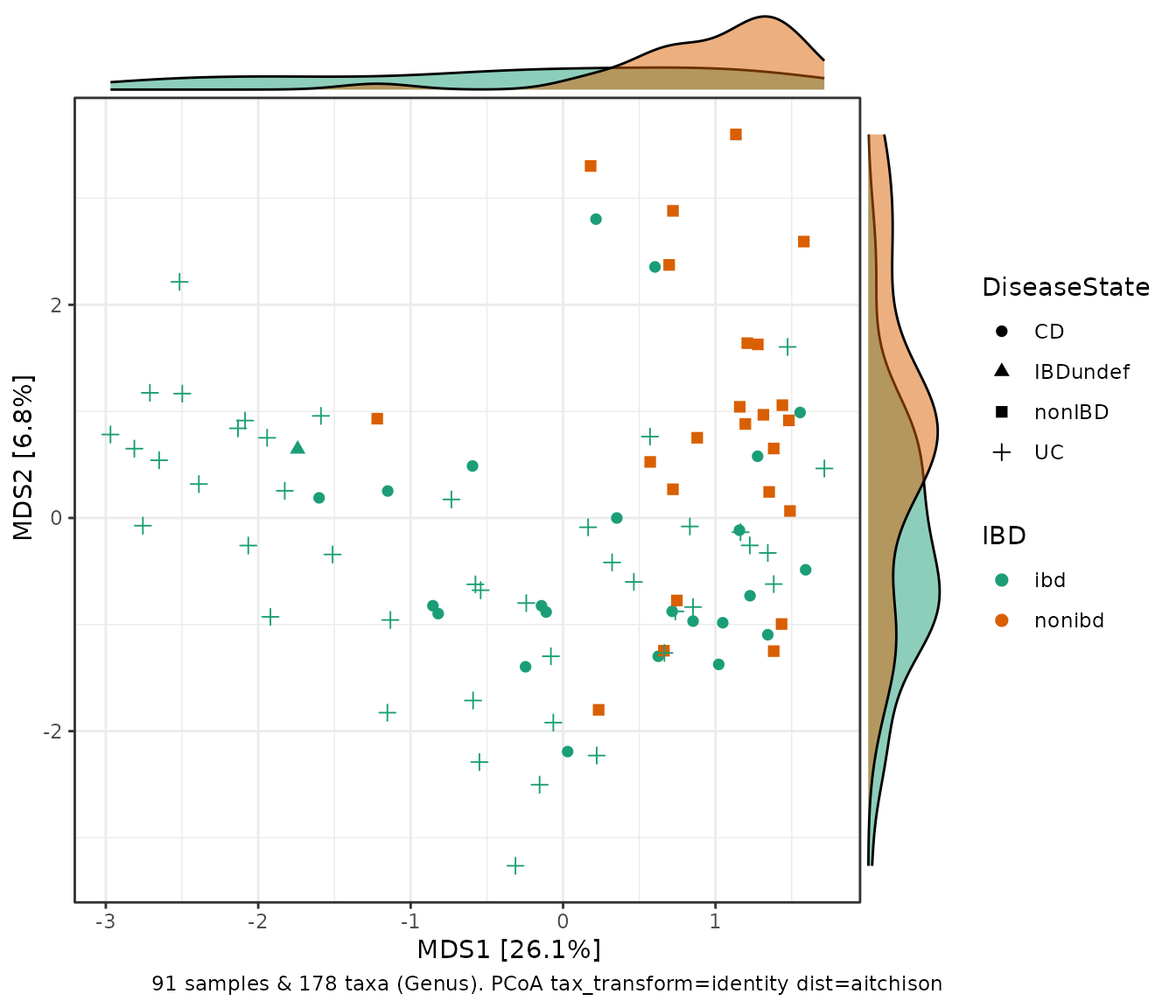
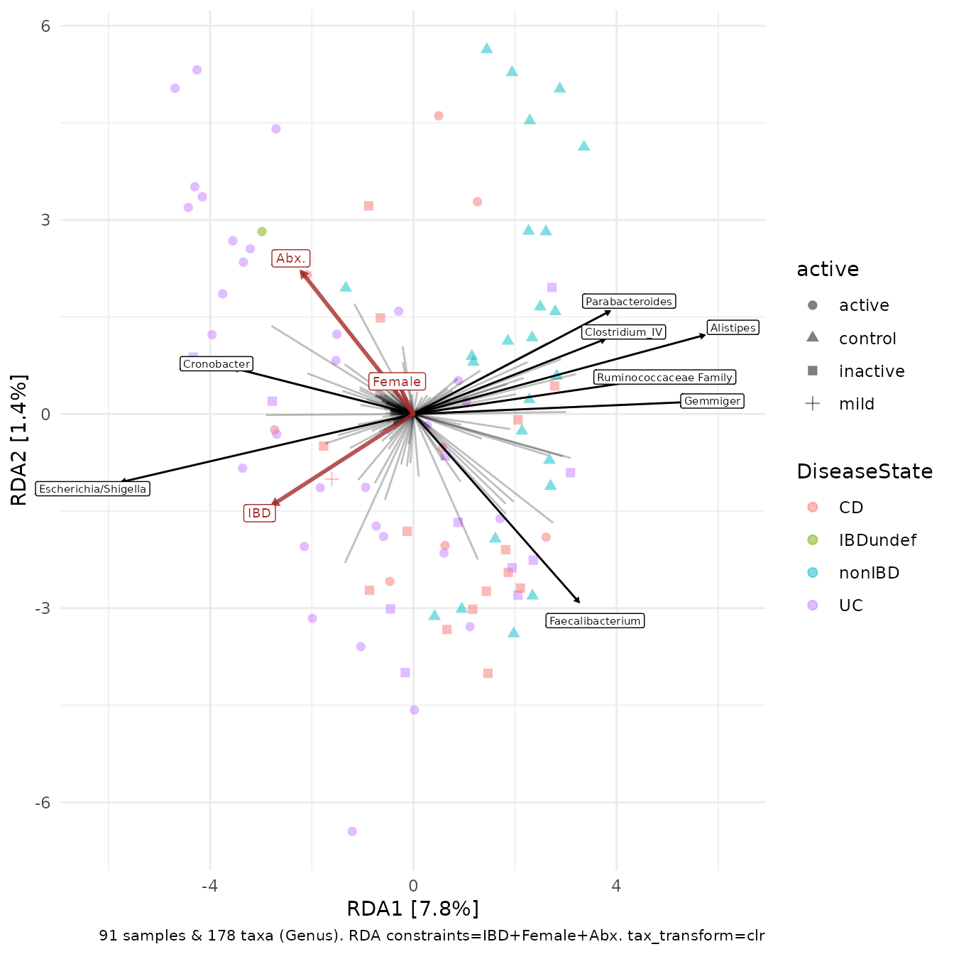
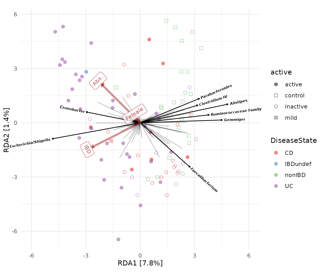
RDA - Redundancy Analysis
Redundancy analysis is a constrained ordination method. It displays the microbial variation that can also be explained by selected constraint variables.
Behind the scenes, a linear regression model is created for each microbial abundance variable (using the constraints as the explanatory variables) and a PCA is performed using the fitted values of the microbial abundances.
Starting from the same phyloseq object ibd the code
below first creates a couple of binary (0/1) numeric variables to use a
constraint variables. This is easy enough with ps_mutate.
Then we aggregate and transform our taxa, and like PCA we skip the dist_calc step.
ibd %>%
  ps_mutate(
    IBD = as.numeric(ibd == "ibd"),
    Female = as.numeric(gender == "female"),
    Abx. = as.numeric(abx == "abx")
  ) %>%
  tax_transform("clr", rank = "Genus") %>%
  ord_calc(
    constraints = c("IBD", "Female", "Abx."),
    # method = "RDA", # Note: you can specify RDA explicitly, and it is good practice to do so, but microViz can guess automatically that you want an RDA here (helpful if you don't remember the name?)
    scale_cc = FALSE # doesn't make a difference
  ) %>%
  ord_plot(
    colour = "DiseaseState", size = 2, alpha = 0.5, shape = "active",
    plot_taxa = 1:8
  )
Customising your ordination plot
The plot above looks okay by default, but it is fairly easy to tweak ord_plot further to get the style just how you want it. The code below has comments to explain which part makes which changes to the plot.
# first we make a function that replaces any unwanted "_" in our taxa labels with spaces
library(stringr)
renamer <- function(x) str_replace(x, pattern = "_", replacement = " ")

ibd %>%
  ps_mutate(
    IBD = as.numeric(ibd == "ibd"),
    Female = as.numeric(gender == "female"),
    Abx. = as.numeric(abx == "abx")
  ) %>%
  tax_transform("clr", rank = "Genus") %>%
  ord_calc(
    constraints = c("IBD", "Female", "Abx."),
    method = "RDA",
    scale_cc = FALSE # doesn't make a difference
  ) %>%
  ord_plot(
    colour = "DiseaseState", size = 2, alpha = 0.5, shape = "active",
    auto_caption = NA, # remove the helpful automatic caption
    plot_taxa = 1:8, taxon_renamer = renamer, # renamer is the function we made earlier
    tax_vec_length = 5, # this value is a scalar multiplier for the biplot score vectors
    tax_lab_length = 6, # this multiplier moves the labels, independently of the arrowheads
    tax_lab_style = tax_lab_style(size = 1.8, alpha = 0.5), # create a list of options to tweak the taxa labels' default style
    constraint_vec_length = 3, # this adjusts the length of the constraint arrows, and the labels track these lengths by default
    constraint_vec_style = vec_constraint(1.5, alpha = 0.5), # this styles the constraint arrows
    constraint_lab_style = constraint_lab_style(size = 3) # this styles the constraint labels
  ) +
  # the functions below are from ggplot2:
  # You can pick a different colour scale, such as a color_brewer palette
  scale_colour_brewer(palette = "Set1") +
  # You can set any scale's values manually, such as the shapes used
  scale_shape_manual(values = c(
    active = "circle", mild = "circle cross",
    inactive = "circle open", control = "square open"
  )) +
  # this is how you add a title and subtitle
  ggtitle(
    label = "[Insert your exciting interpretations here?]",
    subtitle = "RDA with clr-transformed genera: constraints in red, taxa in black"
  ) +
  # and this is how you make your own caption
  labs(caption = "91 samples, 178 genera. Type 2 scaling.") +
  # this is one way to set the aspect ratio of the plot
  coord_fixed(ratio = 1, clip = "off")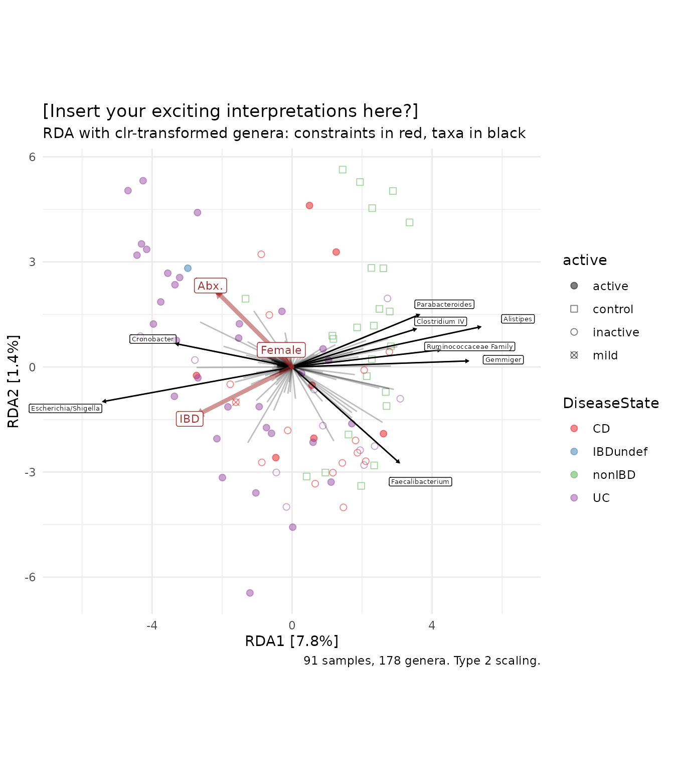
Custom labels
tax_lab_style() is a helper function that gives you some
options for customising the look of the taxa loading labels, including,
in this example, using rotated, bold and italic text for the taxa
names.
constraint_lab_style() is a similar helper function for
customising the constraint labels. When rotating labels (not text) the
ggtext package must be installed.
ibd %>%
  ps_mutate(
    IBD = as.numeric(ibd == "ibd"),
    Female = as.numeric(gender == "female"),
    Abx. = as.numeric(abx == "abx")
  ) %>%
  tax_transform("clr", rank = "Genus") %>%
  ord_calc(
    constraints = c("IBD", "Female", "Abx."),
    method = "RDA",
    scale_cc = FALSE # doesn't make a difference
  ) %>%
  ord_plot(
    colour = "DiseaseState", size = 2, alpha = 0.5, shape = "active",
    auto_caption = NA,
    plot_taxa = 1:8, taxon_renamer = renamer,
    # with rotated labels, it is nicer to keep lab_length closer to vec_length
    tax_vec_length = 4.5, tax_lab_length = 4.6,
    tax_lab_style = tax_lab_style(
      type = "text", max_angle = 90, fontface = "bold.italic"
    ),
    constraint_vec_style = vec_constraint(1.5, alpha = 0.5),
    constraint_vec_length = 3, constraint_lab_length = 3.3,
    constraint_lab_style = constraint_lab_style(
      alpha = 0.8, size = 3, max_angle = 90, perpendicular = TRUE
    )
  ) +
  # SETTING A FIXED RATIO IDENTICAL TO THE aspect_ratio ARGUMENT IN
  # tax_lab_style() IS NECESSARY FOR THE ANGLES OF TEXT TO ALIGN WITH ARROWS!
  coord_fixed(ratio = 1, clip = "off", xlim = c(-6, 6)) +
  # The scales below are set the same as in the previous customisation:
  scale_colour_brewer(palette = "Set1") +
  scale_shape_manual(values = c(
    active = "circle", mild = "circle cross",
    inactive = "circle open", control = "square open"
  ))
Partial ordinations
Tutorial coming soon, for now see ord_plot() for
examples.
Session info
devtools::session_info()
#> ─ Session info ───────────────────────────────────────────────────────────────
#>  setting  value
#>  version  R version 4.6.0 (2026-04-24)
#>  os       Ubuntu 24.04.4 LTS
#>  system   x86_64, linux-gnu
#>  ui       X11
#>  language en
#>  collate  C.UTF-8
#>  ctype    C.UTF-8
#>  tz       UTC
#>  date     2026-06-01
#>  pandoc   3.8.3 @ /opt/hostedtoolcache/pandoc/3.8.3/x64/ (via rmarkdown)
#>  quarto   NA
#>
#> ─ Packages ───────────────────────────────────────────────────────────────────
#>  package      * version   date (UTC) lib source
#>  ade4           1.7-24    2026-03-21 [1] RSPM
#>  ape            5.8-1     2024-12-16 [1] RSPM
#>  Biobase        2.72.0    2026-04-28 [1] Bioconduc~
#>  BiocGenerics   0.58.1    2026-05-14 [1] Bioconduc~
#>  biomformat     1.40.0    2026-04-28 [1] Bioconduc~
#>  Biostrings     2.80.1    2026-05-22 [1] Bioconduc~
#>  bslib          0.11.0    2026-05-16 [1] RSPM
#>  cachem         1.1.0     2024-05-16 [1] RSPM
#>  cli            3.6.6     2026-04-09 [1] RSPM
#>  clue           0.3-68    2026-03-26 [1] RSPM
#>  cluster        2.1.8.2   2026-02-05 [3] CRAN (R 4.6.0)
#>  codetools      0.2-20    2024-03-31 [3] CRAN (R 4.6.0)
#>  commonmark     2.0.0     2025-07-07 [1] RSPM
#>  crayon         1.5.3     2024-06-20 [1] RSPM
#>  data.table     1.18.4    2026-05-06 [1] RSPM
#>  desc           1.4.3     2023-12-10 [1] RSPM
#>  devtools       2.5.2     2026-04-30 [1] RSPM
#>  digest         0.6.39    2025-11-19 [1] RSPM
#>  dplyr          1.2.1     2026-04-03 [1] RSPM
#>  ellipsis       0.3.3     2026-04-04 [1] RSPM
#>  evaluate       1.0.5     2025-08-27 [1] RSPM
#>  farver         2.1.2     2024-05-13 [1] RSPM
#>  fastmap        1.2.0     2024-05-15 [1] RSPM
#>  fBasics        4052.98   2025-12-07 [1] RSPM
#>  foreach        1.5.2     2022-02-02 [1] RSPM
#>  fs             2.1.0     2026-04-18 [1] RSPM
#>  generics       0.1.4     2025-05-09 [1] RSPM
#>  ggplot2      * 4.0.3     2026-04-22 [1] RSPM
#>  ggrepel        0.9.8     2026-03-17 [1] RSPM
#>  ggside         0.4.1     2025-11-25 [1] RSPM
#>  ggtext         0.1.2     2022-09-16 [1] RSPM
#>  glue           1.8.1     2026-04-17 [1] RSPM
#>  gridtext       0.1.6     2026-02-19 [1] RSPM
#>  gtable         0.3.6     2024-10-25 [1] RSPM
#>  GUniFrac       1.9       2025-08-25 [1] RSPM
#>  htmltools      0.5.9     2025-12-04 [1] RSPM
#>  htmlwidgets    1.6.4     2023-12-06 [1] RSPM
#>  igraph         2.3.2     2026-05-29 [1] RSPM
#>  inline         0.3.21    2025-01-09 [1] RSPM
#>  IRanges        2.46.0    2026-04-28 [1] Bioconduc~
#>  iterators      1.0.14    2022-02-05 [1] RSPM
#>  jquerylib      0.1.4     2021-04-26 [1] RSPM
#>  jsonlite       2.0.0     2025-03-27 [1] RSPM
#>  knitr          1.51      2025-12-20 [1] RSPM
#>  labeling       0.4.3     2023-08-29 [1] RSPM
#>  lattice        0.22-9    2026-02-09 [3] CRAN (R 4.6.0)
#>  lifecycle      1.0.5     2026-01-08 [1] RSPM
#>  litedown       0.9       2025-12-18 [1] RSPM
#>  magrittr       2.0.5     2026-04-04 [1] RSPM
#>  markdown       2.0       2025-03-23 [1] RSPM
#>  MASS           7.3-65    2025-02-28 [3] CRAN (R 4.6.0)
#>  Matrix         1.7-5     2026-03-21 [3] CRAN (R 4.6.0)
#>  matrixStats    1.5.0     2025-01-07 [1] RSPM
#>  memoise        2.0.1     2021-11-26 [1] RSPM
#>  mgcv           1.9-4     2025-11-07 [3] CRAN (R 4.6.0)
#>  microbiome     1.34.0    2026-04-28 [1] Bioconduc~
#>  microViz     * 0.13.1    2026-06-01 [1] local
#>  modeest        2.4.0     2019-11-18 [1] RSPM
#>  multtest       2.68.0    2026-04-28 [1] Bioconduc~
#>  nlme           3.1-169   2026-03-27 [3] CRAN (R 4.6.0)
#>  otel           0.2.0     2025-08-29 [1] RSPM
#>  patchwork      1.3.2     2025-08-25 [1] RSPM
#>  permute        0.9-10    2026-02-06 [1] RSPM
#>  phyloseq     * 1.56.0    2026-04-28 [1] Bioconduc~
#>  pillar         1.11.1    2025-09-17 [1] RSPM
#>  pkgbuild       1.4.8     2025-05-26 [1] RSPM
#>  pkgconfig      2.0.3     2019-09-22 [1] RSPM
#>  pkgdown        2.2.0     2025-11-06 [1] RSPM
#>  pkgload        1.5.2     2026-04-22 [1] RSPM
#>  plyr           1.8.9     2023-10-02 [1] RSPM
#>  purrr          1.2.2     2026-04-10 [1] RSPM
#>  R6             2.6.1     2025-02-15 [1] RSPM
#>  ragg           1.5.2     2026-03-23 [1] RSPM
#>  RColorBrewer   1.1-3     2022-04-03 [1] RSPM
#>  Rcpp           1.1.1-1.1 2026-04-24 [1] RSPM
#>  reshape2       1.4.5     2025-11-12 [1] RSPM
#>  rlang          1.2.0     2026-04-06 [1] RSPM
#>  rmarkdown      2.31      2026-03-26 [1] RSPM
#>  rmutil         1.1.10    2022-10-27 [1] RSPM
#>  rpart          4.1.27    2026-03-27 [3] CRAN (R 4.6.0)
#>  Rtsne          0.17      2023-12-07 [1] RSPM
#>  S4Vectors      0.50.1    2026-05-13 [1] Bioconduc~
#>  S7             0.2.2     2026-04-22 [1] RSPM
#>  sass           0.4.10    2025-04-11 [1] RSPM
#>  scales         1.4.0     2025-04-24 [1] RSPM
#>  Seqinfo        1.2.0     2026-04-28 [1] Bioconduc~
#>  sessioninfo    1.2.3     2025-02-05 [1] RSPM
#>  spatial        7.3-18    2025-01-01 [3] CRAN (R 4.6.0)
#>  stable         1.1.7     2026-02-15 [1] RSPM
#>  stabledist     0.7-2     2024-08-17 [1] RSPM
#>  statip         0.2.3     2019-11-17 [1] RSPM
#>  statmod        1.5.2     2026-05-17 [1] RSPM
#>  stringi        1.8.7     2025-03-27 [1] RSPM
#>  stringr      * 1.6.0     2025-11-04 [1] RSPM
#>  survival       3.8-6     2026-01-16 [3] CRAN (R 4.6.0)
#>  systemfonts    1.3.2     2026-03-05 [1] RSPM
#>  textshaping    1.0.5     2026-03-06 [1] RSPM
#>  tibble         3.3.1     2026-01-11 [1] RSPM
#>  tidyr          1.3.2     2025-12-19 [1] RSPM
#>  tidyselect     1.2.1     2024-03-11 [1] RSPM
#>  timeDate       4052.112  2026-01-28 [1] RSPM
#>  timeSeries     4052.112  2025-12-12 [1] RSPM
#>  usethis        3.2.1     2025-09-06 [1] RSPM
#>  vctrs          0.7.3     2026-04-11 [1] RSPM
#>  vegan          2.7-5     2026-05-25 [1] RSPM
#>  withr          3.0.2     2024-10-28 [1] RSPM
#>  xfun           0.57      2026-03-20 [1] RSPM
#>  xml2           1.5.2     2026-01-17 [1] RSPM
#>  XVector        0.52.0    2026-04-28 [1] Bioconduc~
#>  yaml           2.3.12    2025-12-10 [1] RSPM
#>
#>  [1] /home/runner/work/_temp/Library
#>  [2] /opt/R/4.6.0/lib/R/site-library
#>  [3] /opt/R/4.6.0/lib/R/library
#>  * ── Packages attached to the search path.
#>
#> ──────────────────────────────────────────────────────────────────────────────