Plot statistical model results for all taxa on a taxonomic tree

Uses a psExtra object to make a tree graph structure from the taxonomic table.
Then adds statistical results stored in "taxatree_stats" of psExtra data
You must use taxatree_models() first to generate statistical model results.
You can adjust p-values with taxatree_stats_p_adjust()

Usage

taxatree_plots(
  data,
  colour_stat = "estimate",
  palette = "Green-Brown",
  reverse_palette = FALSE,
  colour_lims = NULL,
  colour_oob = scales::oob_squish,
  colour_trans = "abs_sqrt",
  size_stat = list(prevalence = prev),
  node_size_range = c(1, 4),
  edge_width_range = node_size_range * 0.8,
  size_guide = "legend",
  size_trans = "identity",
  sig_stat = "p.value",
  sig_threshold = 0.05,
  sig_shape = "circle filled",
  sig_size = 0.75,
  sig_stroke = 0.75,
  sig_colour = "white",
  edge_alpha = 0.7,
  vars = "term",
  var_renamer = identity,
  title_size = 10,
  layout = "tree",
  layout_seed = NA,
  circular = identical(layout, "tree"),
  node_sort = NULL,
  add_circles = isTRUE(circular),
  drop_ranks = TRUE,
  l1 = if (palette == "Green-Brown") 10 else NULL,
  l2 = if (palette == "Green-Brown") 85 else NULL,
  colour_na = "grey35"
)

Arguments

data: psExtra with taxatree_stats, e.g. output of taxatree_models2stats()
colour_stat: name of variable to scale colour/fill of nodes and edges
palette: diverging hcl colour palette name from colorspace::hcl_palettes("diverging")
reverse_palette: reverse direction of colour palette?
colour_lims: limits of colour and fill scale, NULL will infer lims from range of all data
colour_oob: scales function to handle colour_stat values outside of colour_lims (default simply squishes "out of bounds" values into the given range)
colour_trans: name of transformation for colour scale: default is "abs_sqrt", the square-root of absolute values, but you can use the name of any transformer from the scales package, such as "identity" or "exp"
size_stat: named list of length 1, giving function calculated for each taxon, to determine the size of nodes (and edges). Name used as size legend title.
node_size_range: min and max node sizes, decrease to avoid node overlap
edge_width_range: min and max edge widths
size_guide: guide for node sizes, try "none", "legend" or ggplot2::guide_legend()
size_trans: transformation for size scale you can use (the name of) any transformer from the scales package, such as "identity", "log1p", or "sqrt"
sig_stat: name of variable indicating statistical significance
sig_threshold: value of sig_stat variable indicating statistical significance (below this)
sig_shape: fixed shape for significance marker
sig_size: fixed size for significance marker
sig_stroke: fixed stroke width for significance marker
sig_colour: fixed colour for significance marker (used as fill for filled shapes)
edge_alpha: fixed alpha value for edges
vars: name of column indicating terms in models (one plot made per term)
var_renamer: function to rename variables for plot titles
title_size: font size of title
layout: any ggraph layout, default is "tree"
layout_seed: any numeric, required if a stochastic igraph layout is named
circular: should the layout be circular?
node_sort: sort nodes by "increasing" or "decreasing" size? NULL for no sorting. Use tax_sort() before taxatree_plots() for finer control.
add_circles: add faint concentric circles to plot, behind each rank?
drop_ranks: drop ranks from tree if not included in stats dataframe
l1: Luminance value at the scale endpoints, NULL for palette's default
l2: Luminance value at the scale midpoint, NULL for palette's default
colour_na: colour for NA values in tree. (if unused ranks are not dropped, they will have NA values for colour_stat)

Value

list of ggraph ggplots

Details

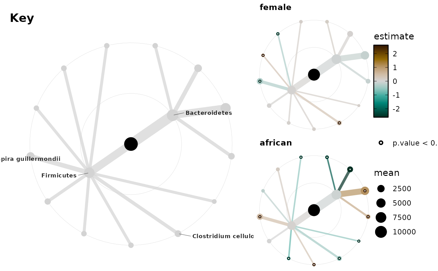
taxatree_plotkey plots same layout as taxatree_plots, but in a fixed colour

See website article for more examples of use: https://david-barnett.github.io/microViz/articles/web-only/modelling-taxa.html

Uses ggraph, see help for main underlying graphing function with ?ggraph::ggraph

It is possible to provide multiple significance markers for multiple thresholds, by passing vectors to the sig_shape, sig_threshold, etc. arguments. It is critically important that the thresholds are provided in decreasing order of severity, e.g. sig_threshold = c(0.001, 0.01, 0.1) and you must provide a shape value for each of them.

Examples

# Limited examples, see website article for more

library(dplyr)
library(ggplot2)

data(dietswap, package = "microbiome")
ps <- dietswap

# create some binary variables for easy visualisation
ps <- ps %>% ps_mutate(
  female = if_else(sex == "female", 1, 0, NaN),
  african = if_else(nationality == "AFR", 1, 0, NaN)
)

# This example dataset has some taxa with the same name for phylum and family...
# We can fix problems like this with the tax_prepend_ranks function
# (This will always happen with Actinobacteria!)
ps <- tax_prepend_ranks(ps)

# filter out rare taxa
ps <- ps %>% tax_filter(
  min_prevalence = 0.5, prev_detection_threshold = 100
)
#> Proportional min_prevalence given: 0.5 --> min 111/222 samples.

# delete the Family rank as we will not use it for this small example
# this is necessary as taxatree_plots can only plot consecutive ranks
ps <- ps %>% tax_mutate(Family = NULL)

# specify variables used for modelling
models <- taxatree_models(
  ps = ps, type = corncob::bbdml, ranks = c("Phylum", "Genus"),
  formula = ~ female + african, verbose = TRUE
)
#> 2025-04-14 11:44:19.48083 - modelling at rank: Phylum
#> Modelling: P: Bacteroidetes
#> Modelling: P: Firmicutes
#> 2025-04-14 11:44:19.627546 - modelling at rank: Genus
#> Modelling: G: Allistipes et rel.
#> Modelling: G: Bacteroides vulgatus et rel.
#> Modelling: G: Butyrivibrio crossotus et rel.
#> Modelling: G: Clostridium cellulosi et rel.
#> Modelling: G: Clostridium orbiscindens et rel.
#> Modelling: G: Clostridium symbiosum et rel.
#> Modelling: G: Faecalibacterium prausnitzii et rel.
#> Modelling: G: Oscillospira guillermondii et rel.
#> Modelling: G: Prevotella melaninogenica et rel.
#> Modelling: G: Prevotella oralis et rel.
#> Modelling: G: Ruminococcus obeum et rel.
#> Modelling: G: Sporobacter termitidis et rel.
#> Modelling: G: Subdoligranulum variable at rel.
# models list stored as attachment in psExtra
models
#> psExtra object - a phyloseq object with extra slots:
#> 
#> phyloseq-class experiment-level object
#> otu_table()   OTU Table:         [ 13 taxa and 222 samples ]
#> sample_data() Sample Data:       [ 222 samples by 10 sample variables ]
#> tax_table()   Taxonomy Table:    [ 13 taxa by 2 taxonomic ranks ]
#> 
#> 
#> taxatree_models list:
#> Ranks: Phylum/Genus

# get stats from models
stats <- taxatree_models2stats(models, param = "mu")
stats
#> psExtra object - a phyloseq object with extra slots:
#> 
#> phyloseq-class experiment-level object
#> otu_table()   OTU Table:         [ 13 taxa and 222 samples ]
#> sample_data() Sample Data:       [ 222 samples by 10 sample variables ]
#> tax_table()   Taxonomy Table:    [ 13 taxa by 2 taxonomic ranks ]
#> 
#> 
#> taxatree_stats dataframe:
#> 15 taxa at 2 ranks: Phylum, Genus 
#> 2 terms: female, african

plots <- taxatree_plots(
  data = stats, colour_trans = "identity",
  size_stat = list(mean = mean),
  size_guide = "legend", node_size_range = c(1, 6)
)

# if you change the size_stat for the plots, do the same for the key!!
key <- taxatree_plotkey(
  data = stats,
  rank == "Phylum" | p.value < 0.05, # labelling criteria
  .combine_label = all, # label only taxa where criteria met for both plots
  size_stat = list(mean = mean),
  node_size_range = c(2, 7), size_guide = "none",
  taxon_renamer = function(x) {
    stringr::str_remove_all(x, "[PG]: | [ae]t rel.")
  }
)

# cowplot is powerful for arranging trees and key and colourbar legend
legend <- cowplot::get_legend(plots[[1]])
#> Warning: Multiple components found; returning the first one. To return all, use `return_all = TRUE`.
plot_col <- cowplot::plot_grid(
  plots[[1]] + theme(legend.position = "none"),
  plots[[2]] + theme(legend.position = "none"),
  ncol = 1
)
cowplot::plot_grid(key, plot_col, legend, nrow = 1, rel_widths = c(4, 2, 1))